Before we’ll jump into understanding and trying to apply an algorithm… I was always wondering what does the word mean? Are we applying it correctly? Is there a history we don’t understand?
In layman’s terms, a computer algorithm is basically a set of processor instructions provided in sequence, which execution stops eventually. It is not a formal definition and most of computer programs would fall within the scope. So if you have ever written a computer program, you wrote an algorithm … Yaay!
This wikipedia article is trying to deal with this problem at length. My favorite citation would be by Mr Kurt Gödel. I will be returning to Kurt and his fantastic thinking in the future on this blog.
“In consequence of later advances, in particular of the fact that, due to A. M. Turing’s work, a precise and unquestionably adequate definition of the general concept of formal system can now be given . . . Turing’s work gives an analysis of the concept of “mechanical procedure” (alias “algorithm” or “computational procedure” or “finite combinatorial procedure”). This concept is shown to be equivalent with that of a “Turing machine”.* A formal system can simply be defined to be any mechanical procedure for producing formulas, called provable formulas . . . .”
(p. 72 in Martin Davis ed. The Undecidable: “Postscriptum” to “On Undecidable Propositions of Formal Mathematical Systems” appearing on p. 39, loc. cit.)
While digging algorithm history a bit deeper, I have found a poetic and cool definition.
Haec algorismus ars praesens dicitur, in qua / Talibus Indorum fruimur bis quinque figuris.
https://commons.wikimedia.org/wiki/File:Carmen_de_Algorismo.pdf
which translates to:
Algorism is the art by which at present we use those Indian figures, which number two times five.
The ‘those Indian figures’ part points to the next step in reviewing where the algorithm may come from. Muhammad ibn Musa al-Khwarizmi was a mathematician living in Baghdad back in the 9th century AD. About 825, al-Khwarizmi wrote a book on the Hindu–Arabic numeral system, which was later translated to Latin in the medieval times. It started with the phrase Dixit Algorizmi (‘Thus spoke Al-Khwarizmi’), where “Algorizmi” was most likely a Latinization of Al-Khwarizmi’s name.
And that settled it for me. Algorithm is basically the name of that guy (just add a few more centuries and a few more Language-inizations).
In computer science we have managed to colloquialize (or bastardize – you choose :) ) algorithm to a very specific meaning. This is an optimized set of instructions, allowing for more efficient execution of a well defined task. This is where terms like binary search, bubble search, selection sort or all of the cryptographic or compression algorithms come from.
Today I’d like to look at a very specific one. Breadth-first search.
Breadth-first search (BFS) is an algorithm for traversing or searching tree or graph data structures. It starts at the tree root (or some arbitrary node of a graph, sometimes referred to as a ‘search key'[1]), and explores all of the neighbor nodes at the present depth prior to moving on to the nodes at the next depth level.
Breadth-first search (BFS) is an algorithm for traversing or searching tree or graph data structures. It starts at the tree root (or some arbitrary node of a graph, sometimes referred to as a ‘search key’), and explores all of the neighbor nodes at the present depth prior to moving on to the nodes at the next depth level.
https://en.wikipedia.org/wiki/Breadth-first_search
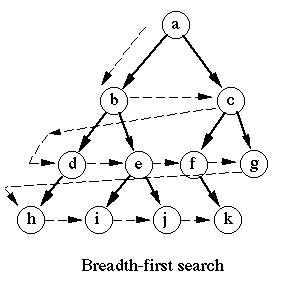
Think of this like standing in front of a column of soldiers (anything can become a ‘tree’ if you’d like to, even a NxN matrix). The line of soldiers you are facing is your breadth. How many rows of soldiers is your depth. Now imagine you are looking for their sergeant and you don’t know in which row/position is he standing. To go breadth-first, select one soldier and scan row by row (you can imagine yourself just going and asking each soldier whether they are sergeant from left to right and then the next row).
Before we proceed it would be good to understand what is time complexity of an algorithm. Cutting the long story short, time complexity is a prediction of how much time the algorithm will take. The second factor to consider is space complexity. This simply deals with the amount of memory required for an algorithm to complete.
You will hear a lot in your career on ‘O’ numbers. Your role in optimization is to keep the O numbers as small as possible, by selecting the right algorithm for the job. Though as today we only learn of one algorithm, let’s leave that for later.
I wouldn’t be myself without touching a bit on history of this algorithm. Specifically on the absolutely wicked word Plankalkül related to it. The year was 1948 and a smart, German scientist – Konrad Zuse had published, what is now deemed the first, complete high-level language. The name translated to English is simply a planning calculator. This is also where BFS was suggested for the first time.
Plankalkül was an attempt by Konrad Zuse in the 1940’s to devise a notational and conceptual system for writing what today is termed a program.
‘The “Plankalkül” of Konrad Zuse: a forerunner of today’s programming languages’ (F.L. Bauer and H. Wössner Mathematisches Institut der Technischen Universität München)
Now to get back on track. Time to do some coding.
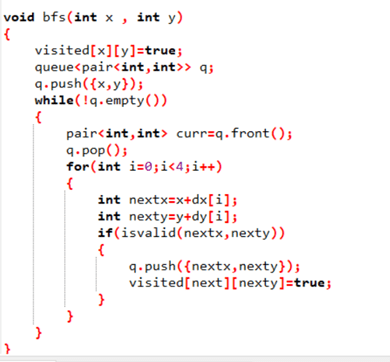
For the coding exercise I have borrowed from the Codingame ‘The Labirynth’ puzzle. BFS is suggested as best-fitted to find a solution to a game with the least number of moves. In my repository, I have created a simple showcase. The main loop of the algorithm is presented below:
   def search(self, start, goal):
        # preparation
        self._prepare_tracking(start)

        # algorithm loop
        while self.queue:
            u = self.queue.pop(0)
            self._review_and_append_forbidden_symbols(goal)
            neighbours = self.map_utils.get_valid_neighbours(self.game_map,self.forbidden_symbols,u)
            for n in neighbours:
                if not self.reviewed[n[0]][n[1]]:
                    self._mark_reviewed(u,n)
                    self.queue.append(n)
                    if self.game_map[n[0]][n[1]] == goal:
                        return self.map_utils.take_step(self.parents, start, n)
        return None
There are a few enhancements here to a typical validation of whether a node in the map matrix is one we can move to. We always strive to look for undiscovered locations to identify the labyrinth ‘exit’. We will never check ‘#’, which is a wall and up until we have run out of undiscovered nodes, we will ignore exit (as we need to go breadth first :)).
This approach was based on this article on BFS and DFS searches. You will probably recognize the similarity to the image below:
Note that in the Codingame task, we are also limited by the max 5×5 visibility field, which makes application of algorithms like Dijkstra’s not likely.
Once you run the algorithm it becomes quite apparent that the people at Codingame had expected BFS to be used, as the alarm limits appear to be matched exactly with the amount of moves you’ll need to execute with the code snippet I had provided.
Time has come to calculate the O numbers. It is not simple to calculate O number of BFS, as it is highly dependent on the graph. Though in this case we get a finite number of max nodes to traverse really, which assumes the memory / space usage is stable. I believe we arrive at linear time and the memory usage is close to constant. But please remember this is just a very simple use-case. Traversing a very large graph with BFS might easily end up with sub-exponential time complexity. Although the algorithm itself is deemed complete (as in it will find a solution – always).
The results of my experiment with performance are listed below:
| Relative graph complexity | Time in s | Space used in kB |
| 14 | .52 | 6700 |
| 42 | .92 | 6996 |
| 208 | 3.18 | 6700 |
| 256 | 2.81 | 6700 |
| 290 | 3.51 | 6700 |
We can then write that in case of our graphs, the time complexity was O(n) and space complexity seems to be O(1).
This is everything I had prepared for today. I always dreaded algorithms and I might actually be one of the developers who prefer to not dwell into the algorithmic thinking. When I get the dread, I then remind myself that:
- a lot of people might never think about what the word algorithm actually means
- in my career (might be nothing to brag about) I have rarely found application of a computer science algorithm, besides knowing them on interviews
- I regularly challenge my knowledge on algorithms on various portals (Codingame being one of them)
Thank you and see you next week!

Leave a comment